Young Eclipsing Binaries
(A more general overview of my research program can be found here.)
Motivation
Eclipsing binary (EB) systems enable precise measurements of stellar masses and radii with minimal model-based assumptions. For this reason, they are ideal objects to benchmark models of stellar evolution. There are relatively few of these systems known at young ages (t < 300 Myr), and as such, there are few reliable benchmarks that are capable of constraining models of pre-main sequence evolution. For this reason, and because pre-main sequence evolution is complicated, there is significant disagreement between models and existing benchmarks, and between different model suites themselves.
This discrepancy highlights that there are physical processes taking place during the formative years of a star’s life that we do not understand, and that current models are unable to capture. They are probably associated to some degree with stellar magnetic fields and star spots. The impact of this short coming is far reaching too – the precision of exoplanet measurements around young stars is limited by our understanding of the stellar host. (See my THYME work as to why we might care about young planets.)
I am working to establish an empirical mass-radius relation across the pre-main sequence using eclipsing binaries. With this work I hope to inform the next generation of stellar evolution models and provide precise relations that will improve the accuracy of exoplanet characterization in young systems. Analyzing these systems necessarily requires confronting the effect of star spots and stellar magnetism. The TESS mission is enabling this work by finding, essentially every near-by short-period eclipsing binary.
Results: TOI 450 – A Young EB in the Columba Association
In the first paper in this series, I have studied TOI 450, a low-mass EB in the 40 Myr Columba association. In the description below I discuss how we confirmed it was a member of Columba, how we modeled the system to include the effect of star spots, and finally, how our measurements compare to models.
A link to the submitted paper can be found here.
Confirming Moving Group Membership
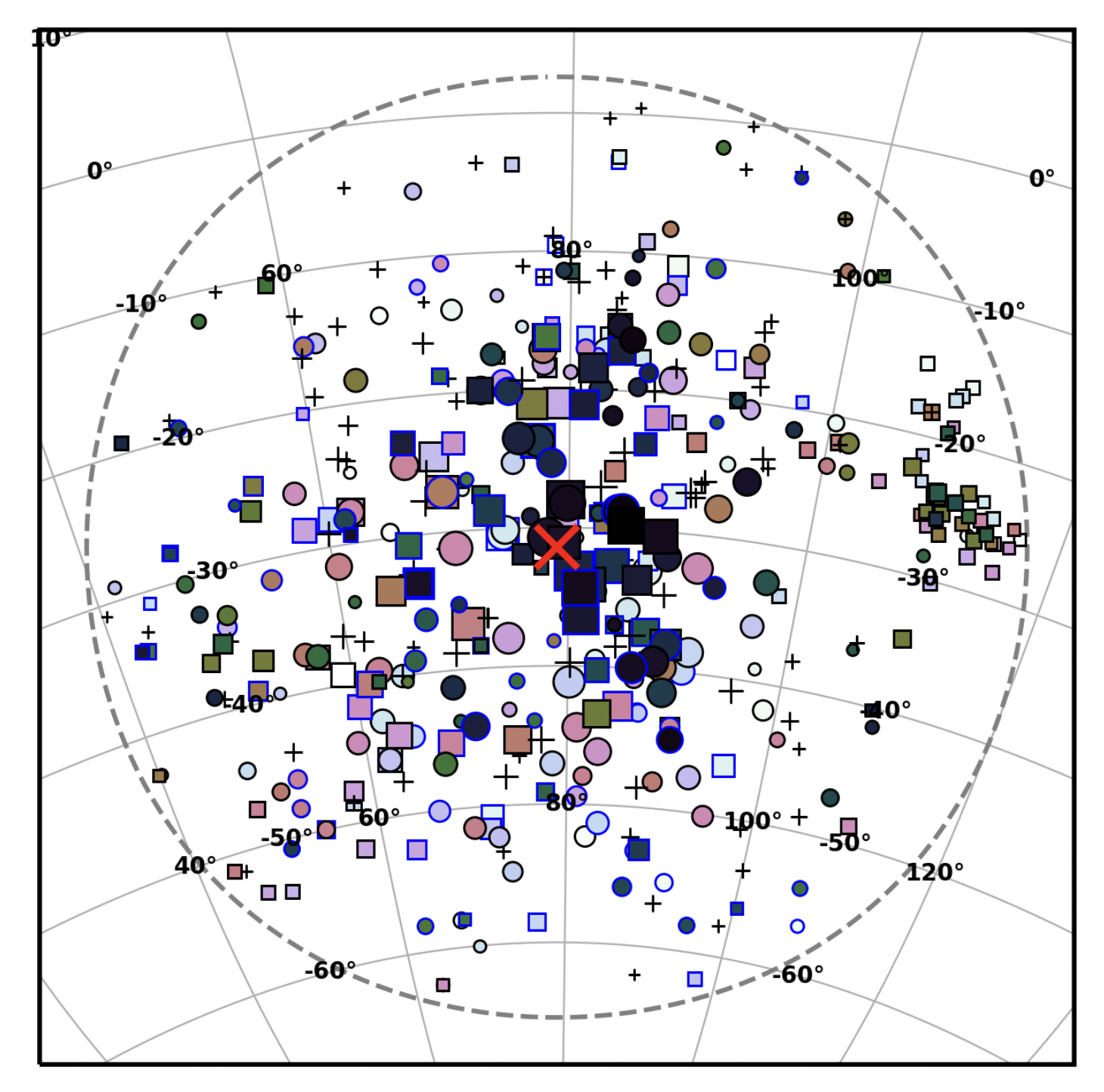
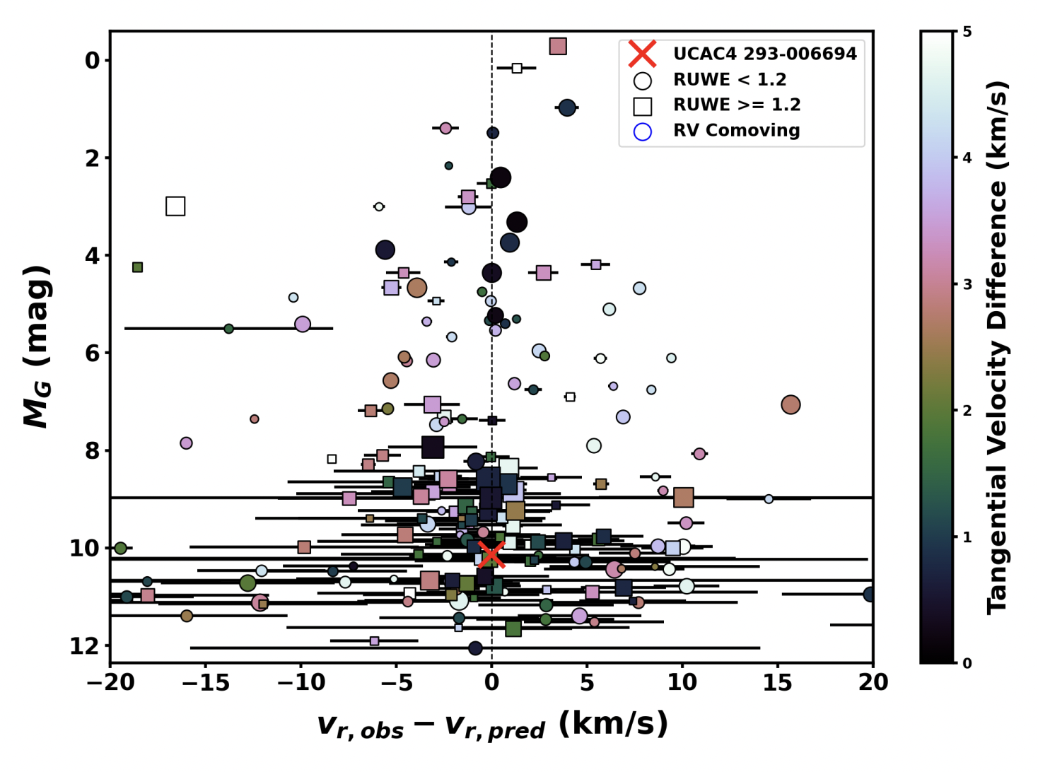
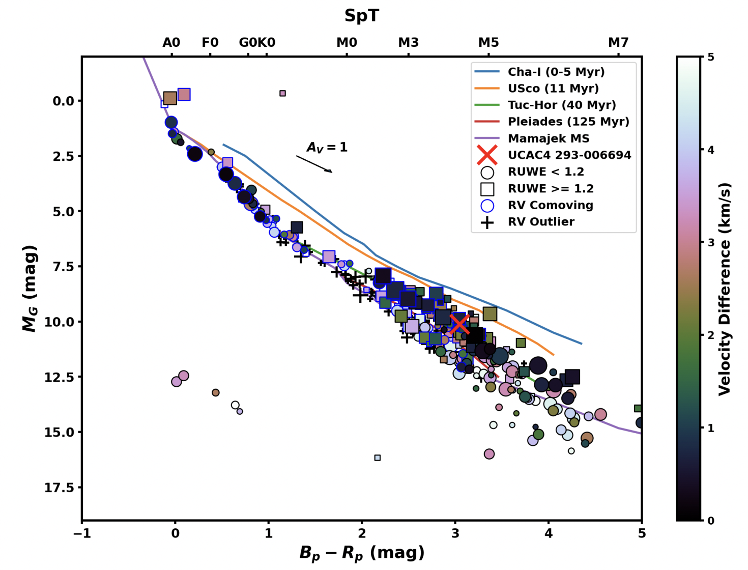
TThe Columba association has a complicated membership history. Many sources, once claimed to be members, have since been ruled out. We wanted to be positive of TOI 450’s membership so we ran the trusty FriendFinder (which you can read more about here). The following three figures summarize the results. First, on the sky, we see a dense collection of stars that are co-distant and co-moving with our binary. Second, we find a majority of these stars are co-moving along the radial direction as well, meaning they share the same motion through the galaxy that was inherited from their parent molecular cloud. And lastly, while contaminated with field stars, we find a sequence of stars that fall along the 40 Myr isochrone. The vast majority of these co-moving members are well-established Columba members, so our work is done! We confirmed TOI 450 is a Columba member and we can now inherit all the precise measurements that come with belonging to a rich stellar ensemble. In our case, we’re mostly interested in age.
Eclipse Fitting and Star Spots
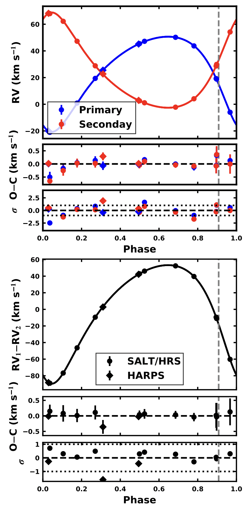
TOI 450 was originally thought to be a planet host because it had one relatively shallow eclipse. Followup spectroscopy showed that it was, in fact, a double-lined spectroscopic binary. In this case the high eccentricity of the orbit conspired with the system’s projection on the sky to provide us with only one grazing eclipse, instead of a primary and secondary eclipse. We do some neat tricks using our high-resolution spectra to place priors on the fit that enable us to characterize the system with a high precision, despite only having one eclipse. I’ll refer you to the paper for that.
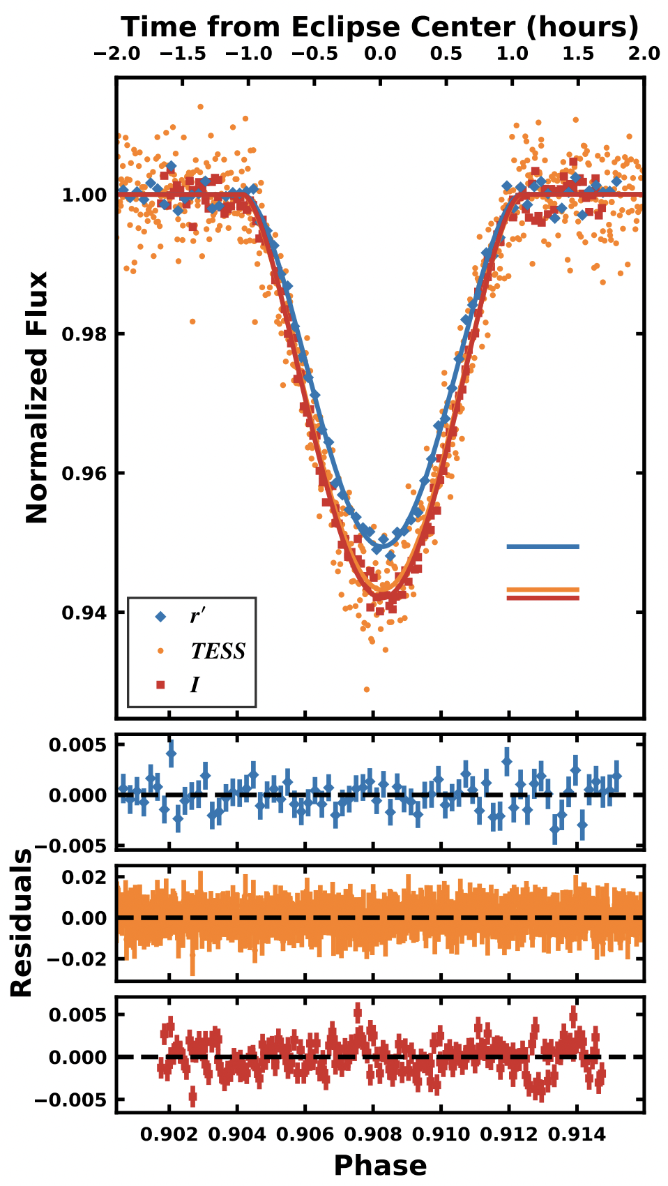
We fit the eclipse light curves and RV measurements simultaneously using an MCMC framework. The neat thing about this data set is that we have multi-color eclipse light curves. You can see in the second figure that the eclipse depth is wavelength dependent. This effect could be due to limb-darkening, but it can also result from eclipsing a region of the star that is more spotted than the disk-integrated average.
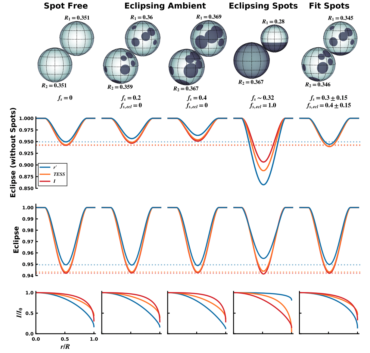
In the figure below I highlight the effect star spots have on eclipse depths. Each column represents a different fit where I make a different assumption about the spots. In the first three columns I gradually increase the spot coverage from 0 to 40%, and assume that the eclipse only passes over ambient photosphere. Each one of these models can reproduce the observed eclipse depths (third row of the figure), but in the absence of spots they correspond to different eclipse depths (second row) and different stellar radii (provided above and below each star in the top row). For reference, the limb-darkening profiles are shown in the bottom row.
Here I am highlighting that the derived radii depend on our assumption about the spot properties, which we essentially have no handle on.
The fourth column assumes the eclipse is only over a completely spotted region, which our multi-color eclipse light curves can rule out. While this model is pathological, we could not strictly rule it out with only one filter.
In the last column we add a new fit parameter to describe the spots in a flexible way, rather than fix them to a certain value. The relevant number here is the spot filling factor of the eclipsed region compared to the disk-integrated average. Here’s how it works:
- If this ratio is one, the eclipse will have the same depth as a spot-free system, regardless of how spotted it actually is.
- If this ratio is less than one, the eclipse will get deeper because the eclipsed area has a larger relative share of the total flux.
- If this ratio is greater than one, the eclipse will get shallower because the eclipsed area has a smaller relative share of the total flux.
With this new formalism, we find that the best fit favors the eclipse passing over a more heavily spotted region than the disk-integrated average, indicating a more polar distribution of spots. Our best fit radii from this model are 2 sigma lower than an unspotted model. This model also has larger radius uncertainty, which is expected given how little we know about the spot distribution. My hope is that this approach will provide a path forward that provides more accurate fundamental parameters and realistic uncertainties.
We ultimately find the stars are “twins”, both having masses of ~0.17 solar masses and radii of 0.345 solar radii, which places these stars firmly on the pre-main sequence.
Comparing to Theoretical Models
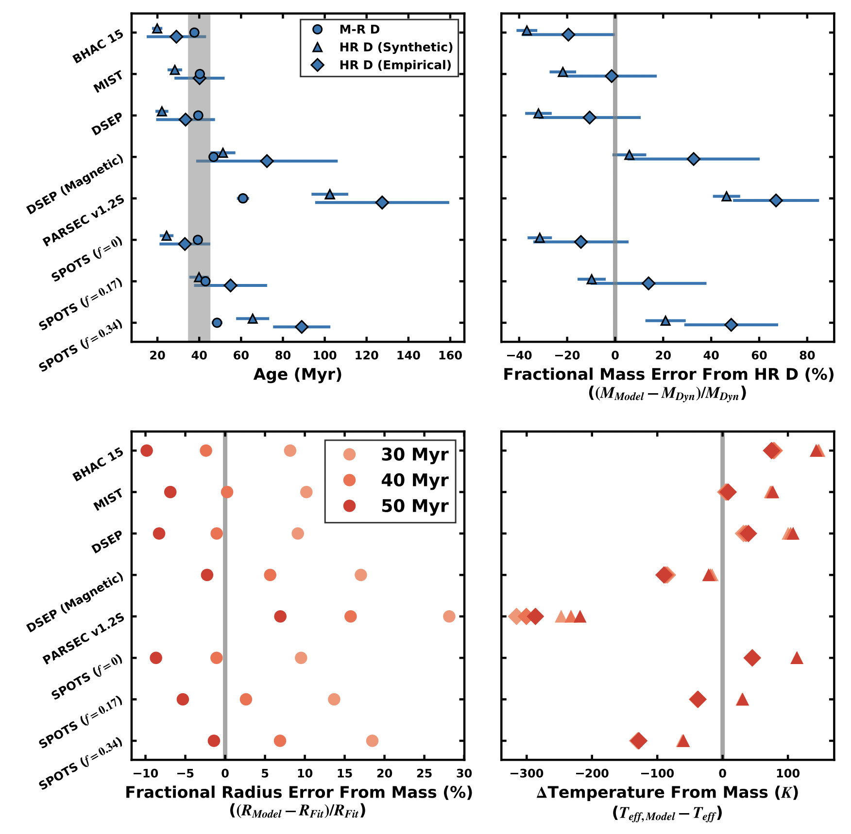
At last, we compare our results to 8 different stellar evolution models. We compare the age derived from our mass and radius measurements with the Columba age (top left). The mass derived from our temperature and luminosity measurements (the HR diagram) are compared with our dynamical measurement (top right). And from our precise mass, we compare model radii and temperatures with our measurements from the SED (bottom left and bottom right, respectively).
The MESA MIST and SPOTS (fs=0.17) isochrones perform the best across our comparisons, but detailed agreement depends heavily on the quantities being compared. Our result is no guarantee that these models will perform well at other masses and ages, but that’s why we’re doing this analysis on lots of young EBs! Stay tuned!

